B Programming in R

When I introduced the idea of working with scripts I said that R starts at the top of the file and runs straight through to the end of the file. That was a tiny bit of a lie. It is true that unless you insert commands to explicitly alter how the script runs, that is what will happen. However, you actually have quite a lot of flexibility in this respect. Depending on how you write the script, you can have R repeat several commands, or skip over different commands, and so on. This topic is referred to as flow control.

B.1 If/else

One kind of flow control that programming languages provide is the ability to evaluate conditional statements. Unlike loops, which can repeat over and over again, a conditional statement only executes once, but it can switch between different possible commands depending on a condition that is specified by the programmer. The power of these commands is that they allow the program itself to make choices, and in particular, to make different choices depending on the context in which the program is run. The most prominent of example of a conditional statement is the if statement, and the accompanying else statement.³⁰

The basic format of an if statement in R is as follows:

if ( CONDITION ) {
  STATEMENT1
  STATEMENT2
  ETC 
}

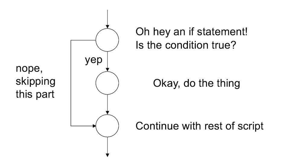
And the execution of the statement is pretty straightforward. If the condition is TRUE, then R will execute the statements contained in the curly braces. If the condition is FALSE, then it does not. So the way R processes an if statement is illustrated by this schematic:

If you want to, you can extend the if statement to include an else statement as well, leading to the following syntax:

if ( CONDITION ) {
  STATEMENT1
  STATEMENT2
  ETC
} else {
  STATEMENT3
  STATEMENT4
  ETC
}

As you’d expect, the interpretation of this version is similar. If the condition is TRUE, then the contents of the first block of code (i.e., statement1, statement2, etc) are executed; but if it is FALSE, then the contents of the second block of code (i.e., statement3, statement4, etc) are executed instead. So the schematic illustration of an if-else construction looks like this:

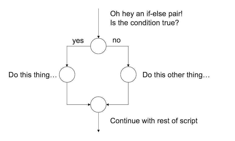
In other words, when we use an if-else pair, we can define different behaviour for our script for both cases.

B.1.1 Example 1:

To give you a feel for how you can use if and else, the example that I’ll show you is a script (feelings.R) that prints out a different message depending the day of the week. Here’s the script:

if(today == "Monday") {
  print("I don’t like Mondays")
} else {
  print("I’m a happy little automaton")
}

So let’s set the value of today to Monday and source the script:

today <- "Monday"
source("./scripts/feelings.R")

## [1] "I don’t like Mondays"

That’s very sad. However, tomorrow should be better:

today <- "Tuesday"
source("./scripts/feelings.R")

## [1] "I’m a happy little automaton"

B.1.2 Example 2:

One useful feature of if and else is that you can chain several of them together to switch between several different possibilities. For example, the more_feelings.R script contains this code:

if(today == "Monday") {
  print("I don’t like Mondays")
  
} else if(today == "Tuesday") {
  print("I’m a happy little automaton")
  
} else if(today == "Wednesday") {
  print("Wednesday is beige")
  
} else {
  print("eh, I have no feelings")
}

B.1.3 Exercises

Write your own version of the “feelings” script that expresses your opinions about summer, winter, autumn and spring. Test your script out.
Expand your script so that it loops over vector of four seasons and prints out your feelings about each of them

The solutions for these exercises are here.

B.2 Loops

The second kind of flow control that I want to talk about is a loop. The idea is simple: a loop is a block of code (i.e., a sequence of commands) that R will execute over and over again until some termination criterion is met. To illustrate the idea, here’s a schematic picture showing the difference between what R does with a script that contains a loop and one that doesn’t:

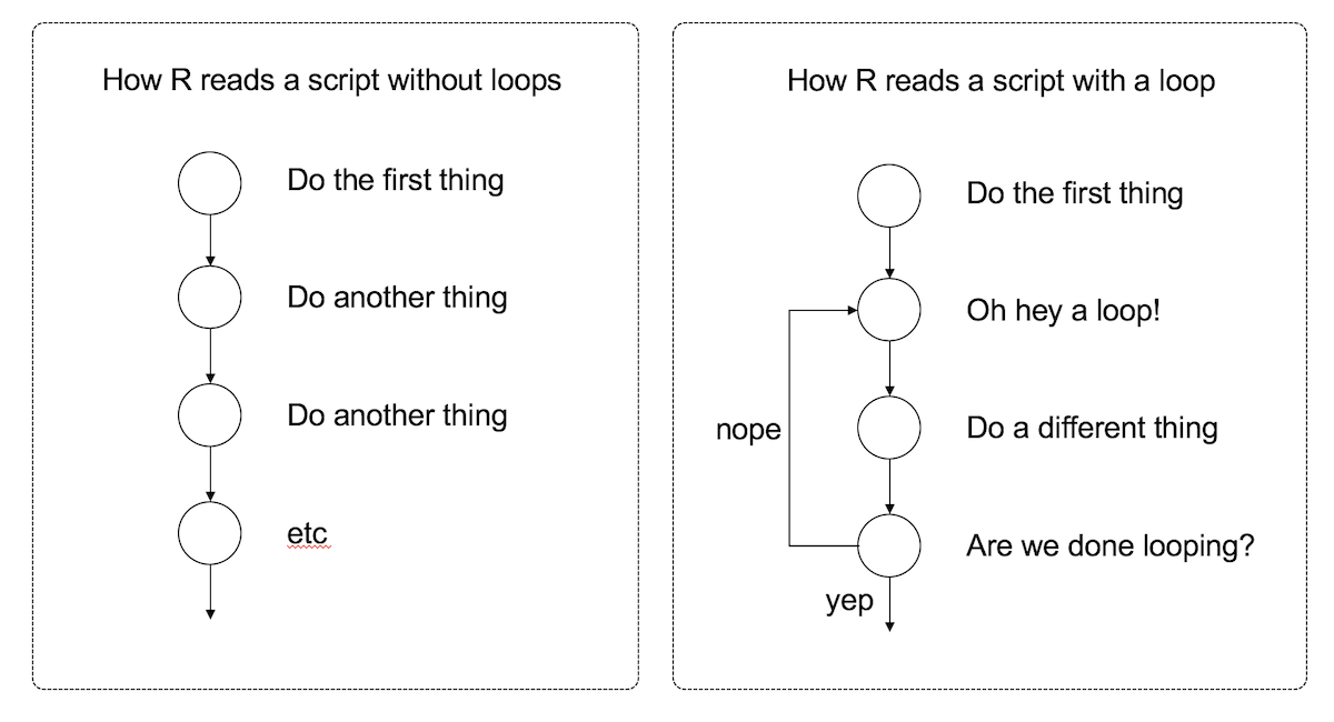
Looping is a very powerful idea, because it allows you to automate repetitive tasks. Much like my children, R will execute an continuous cycle of “are we there yet? are we there yet? are we there yet?” checks against the termination criterion, and it will keep going forever until it is finally there and can break out of the loop. Rather unlike my children, however, I find that this behaviour is actually helpful.

There are several different ways to construct a loop in R. There are two methods I’ll talk about here, one using the while command and another using the for command.

B.2.1 The `while` loop

A while loop is a simple thing. The basic format of the loop looks like this:

while ( CONDITION ) {
  STATEMENT1
  STATEMENT2
  ETC 
}

The code corresponding to condition needs to produce a logical value, either TRUE or FALSE. Whenever R encounters a while statement, it checks to see if the condition is TRUE. If it is, then R goes on to execute all of the commands inside the curly brackets, proceeding from top to bottom as usual. However, when it gets to the bottom of those statements, it moves back up to the while statement. Then, like the mindless automaton it is, it checks to see if the condition is TRUE. If it is, then R goes on to execute all the commands inside … well, you get the idea. This continues endlessly until at some point the condition turns out to be FALSE. Once that happens, R jumps to the bottom of the loop (i.e., to the } character), and then continues on with whatever commands appear next in the script.

B.2.2 A simple example

To start with, let’s keep things simple, and use a while loop to calculate the smallest multiple of 179 that is greater than or equal to 1000. This is of course a very silly example, since you can calculate it using simple arithmetic, but the point here isn’t to do something novel. The point is to show how to write a while loop. Here’s the code in action:

x <- 0
while(x < 1000) {
  x <- x + 179
}
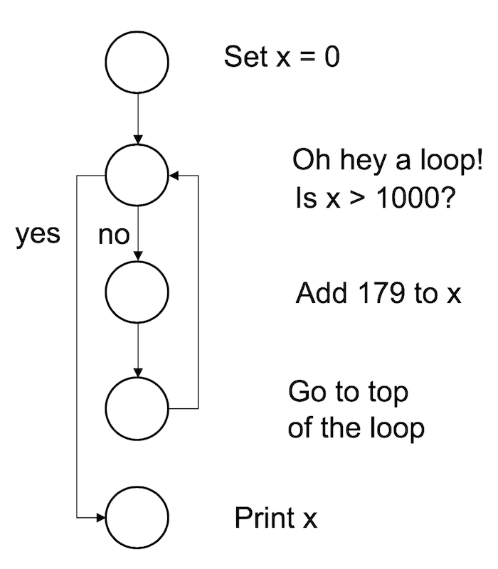
print(x)

## [1] 1074

When we run this code, R starts at the top and creates a new variable called x and assigns it a value of 0. It then moves down to the loop, and “notices” that the condition here is x < 1000. Since the current value of x is zero, the condition is TRUE, so it enters the body of the loop (inside the curly braces). There’s only one command here, which instructs R to increase the value of x by 179. R then returns to the top of the loop, and rechecks the condition. The value of x is now 179, but that’s still less than 1000, so the loop continues. Here’s a visual representation of that:

To see this in action, we can move the print statement inside the body of the loop. By doing that, R will print out the value of x every time it gets updated. Let’s watch:

x <- 0
while(x < 1000) {
  x <- x + 179
  print(x)
}

## [1] 179
## [1] 358
## [1] 537
## [1] 716
## [1] 895
## [1] 1074

Truly fascinating stuff.

B.2.3 Mortgage calculator

To give you a sense of how you can use a while loop in a more complex situation, let’s write a simple script to simulate the progression of a mortgage. BLEGH COME UP WITH SOMETHING BETTER

A happy ending! Yaaaaay!

B.2.4 The `for` loop

The for loop is also pretty simple, though not quite as simple as the while loop. The basic format of this loop goes like this:

for ( VAR in VECTOR ) {
  STATEMENT1
  STATEMENT2
  ETC 
}

In a for loop, R runs a fixed number of iterations. We have a vector which has several elements, each one corresponding to a possible value of the variable var. In the first iteration of the loop, var is given a value corresponding to the first element of vector; in the second iteration of the loop var gets a value corresponding to the second value in vector; and so on. Once we’ve exhausted all of the values in the vector, the loop terminates and the flow of the program continues down the script.

B.2.5 Multiplication tables

When I was a kid we used to have multiplication tables hanging on the walls at home, so I’d end up memorising the all the multiples of small numbers. I was okay at this as long as all the numbers were smaller than 10. Anything above that and I got lazy. So as a first example we’ll get R to print out the multiples of 137. Let’s say I want to it to calculate \(137 \times 1\), then \(137 \times 2\), and so on until we reach \(137 \times 10\). In other words what we want to do is calculate 137 * value for every value within the range spanned by 1:10, and then print the answer to the console. Because we have a fixed range of values that we want to loop over, this situation is well-suited to a for loop. Here’s the code:

for(value in 1:10) {
  answer <- 137 * value
  print(answer)
}

## [1] 137
## [1] 274
## [1] 411
## [1] 548
## [1] 685
## [1] 822
## [1] 959
## [1] 1096
## [1] 1233
## [1] 1370

The intuition here is that R starts by setting value to 1. It then computes and prints 137 * value, then moves back to the top of the loop. When it gets there, it increases value by 1, and then repeats the calculation. It keeps doing this until the value reaches 10 and then it stops. That intuition is essentially correct, but it’s worth unpacking it a bit further using a different example where R loops over something other than a sequence of numbers…

B.2.6 Looping over other vectors

In the example above, the for loop was defined over the numbers from 1 to 10, specified using the R code 1:10. However, it’s worth keeping in mind that as far as R is concerned, 1:10 is actually a vector:

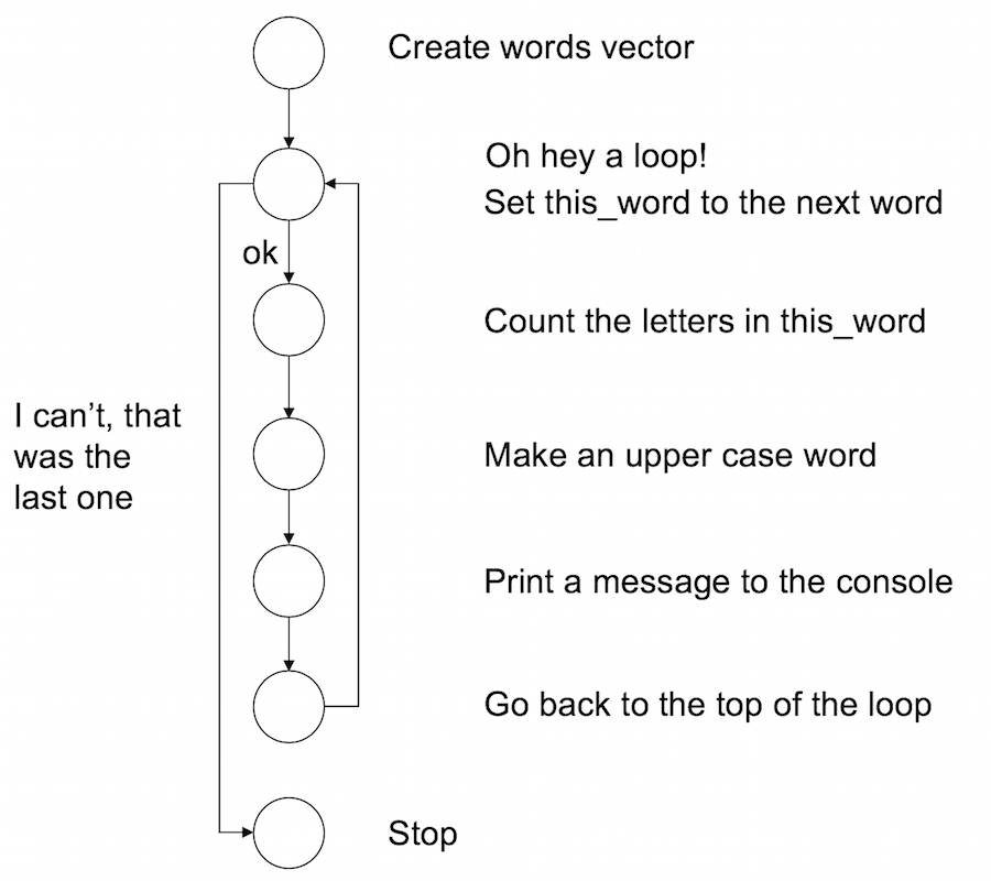
1:10

##  [1]  1  2  3  4  5  6  7  8  9 10

So in the previous example, the intuition about the for loop is slightly misleading. When R gets to the top of the loop the action it takes is “assigning value equal to the next element of the vector”. In this case it turns out that this action causes R to “increase value by 1”, but that’s not true in general. To illustrate that, here’s an example in which a for loop iterates over a character vector. First, I’ll create a vector of words:

words <- c("it", "was", "the", "dirty", "end", "of", "winter")

Now what I’ll do is create a for loop using this vector. For every word in the vector of words R will do three things:

Count the number of letters in the word
Convert the word to upper case
Print a nice summary to the console

Here it is:

for(this_word in words) {
  n_letters <- nchar(this_word)
  block_word <- toupper(this_word)
  cat(block_word, "has", n_letters, "letters\n")
}

## IT has 2 letters
## WAS has 3 letters
## THE has 3 letters
## DIRTY has 5 letters
## END has 3 letters
## OF has 2 letters
## WINTER has 6 letters

From the perspective of the R interpreter this is what the code four the for loop is doing. It’s pretty similar to the while loop, but not quite the same:

B.2.7 Vectorised code?

Somebody has to write loops: it doesn’t have to be you - Jenny Bryan

Of course, there are ways of doing this that don’t require you to write the loop manually. Because many functions in R operate naturally on vectors, you can take advantage of this. Code that bypasses the need to write loops is called vectorised code, and there are some good reasons to do this (sometimes) once you’re comfortable working in R. Here’s an example:

chars <- nchar(words)
names(chars) <- toupper(words)
print(chars)

##     IT    WAS    THE  DIRTY    END     OF WINTER 
##      2      3      3      5      3      2      6

Sometimes vectorised code is easy to write and easy to read. I think the example above is pretty simple, for instance. It’s not always so easy though!

When you go out into the wider world of R programming you’ll probably encounter a lot of examples of people talking about how to vectorise your code to produce better performance. My advice for novices is not to worry about that right now. Loops are perfectly fine, and it’s often more intuitive to write code using loops than using vectors. Eventually you’ll probably want to think about these topics but it’s something that you can leave for a later date!

B.2.8 Exercises

To start with, here are some exercises with for loops and turtles: [WE’RE DROPPING TURTLES]

Use TurtleGraphics to draw a square rather than a hexagon
Use TurtleGraphics to draw a triangle.
Is there a way in which you can get R to automatically work out the angle rather than you having to manually work it out?

As an exercise in using a while loop, consider this vector:

telegram <- c("All","is","well","here","STOP","This","is","fine")

Write a while loop that prints words from telegram until it reaches STOP. When it encounters the word STOP, end the loop. So what you want is output that looks like this.

## [1] "All"
## [1] "is"
## [1] "well"
## [1] "here"
## [1] "STOP"

B.3 Functions

In this section I want to talk about functions again. We’ve been using functions from the beginning, but you’ve learned a lot about R since then, so we can talk about them in more detail. In particular, I want to show you how to create your own. To stick with the same basic framework that I used to describe loops and conditionals, here’s the syntax that you use to create a function:

FNAME <- function( ARG1, ARG2, ETC ) {
  STATEMENT1
  STATEMENT2
  ETC
  return( VALUE )
}

What this does is create a function with the name fname, which has arguments arg1, arg2 and so forth. Whenever the function is called, R executes the statements in the curly braces, and then outputs the contents of value to the user. Note, however, that R does not execute the function commands inside the workspace. Instead, what it does is create a temporary local environment: all the internal statements in the body of the function are executed there, so they remain invisible to the user. Only the final results in the value are returned to the workspace.

B.3.1 A boring example

To give a simple example of this, let’s create a function called quadruple which multiplies its inputs by four.

quadruple <- function(x) {
  y <- x * 4
  return(y)
}

When we run this command, nothing happens apart from the fact that a new object appears in the workspace corresponding to the quadruple function. Not surprisingly, if we ask R to tell us what kind of object it is, it tells us that it is a function:

class(quadruple)

## [1] "function"

And now that we’ve created the quadruple() function, we can call it just like any other function:

quadruple(10)

## [1] 40

An important thing to recognise here is that the two internal variables that the quadruple function makes use of, x and y, stay internal. At no point do either of these variables get created in the workspace.

B.3.2 Default arguments

Okay, now that we are starting to get a sense for how functions are constructed, let’s have a look at a slightly more complex example. Consider this function:

pow <- function(x, y = 1) { 
  out <- x ^ y  # raise x to the power y 
  return(out)
}

The pow function takes two arguments x and y, and computes the value of \(x^y\). For instance, this command

pow(x = 4, y = 2)

## [1] 16

computes 4 squared. The interesting thing about this function isn’t what it does, since R already has has perfectly good mechanisms for calculating powers. Rather, notice that when I defined the function, I specified y=1 when listing the arguments? That’s the default value for y. So if we enter a command without specifying a value for y, then the function assumes that we want y=1:

pow(x = 3)

## [1] 3

However, since I didn’t specify any default value for x when I defined the pow function, the user must input a value for x or else R will spit out an error message.

B.3.3 Unspecified arguments

The other thing I should point out while I’m on this topic is the use of the ... argument. The ... argument is a special construct in R which is only used within functions. It is used as a way of matching against multiple user inputs: in other words, ... is used as a mechanism to allow the user to enter as many inputs as they like. I won’t talk at all about the low-level details of how this works at all, but I will show you a simple example of a function that makes use of it. Consider the following:

doubleMax <- function(...) {
  max.val <- max(...)  # find the largest value in ...
  out <- 2 * max.val   # double it
  return(out)
}

The doubleMax function doesn’t do anything with the user input(s) other than pass them directly to the max function. You can type in as many inputs as you like: the doubleMax function identifies the largest value in the inputs, by passing all the user inputs to the max function, and then doubles it. For example:

doubleMax(1, 2, 5)

## [1] 10

B.3.4 More on functions?

There’s a lot of other details to functions that I’ve hidden in my description in this chapter. Experienced programmers will wonder exactly how the scoping rules work in R, or want to know how to use a function to create variables in other environments, or if function objects can be assigned as elements of a list and probably hundreds of other things besides. However, I don’t want to have this discussion get too cluttered with details, so I think it’s best – at least for the purposes of the current book – to stop here.

B.4 Rescorla-Wagner model

At this point you have all the tools you need to write a fully functional R program. To illustrate this, let’s write a program that implements the Rescorla-Wagner model of associative learning, and apply it to a few simple experimental designs.

B.4.1 The model itself

The Rescorla-Wagner model provides a learning rule that describes how associative strength changes during Pavlovian conditioning. Suppose we take an initially neutral stimulus (e.g., a tone), and pair it with an outcome that has inherent value to the organism (e.g., food, shock). Over time the organism learns to associate the tone with the shock and will respond to the tone in much the same way that it does to the shock. In this example the shock is referred to as the unconditioned stimulus (US) and the tone is the conditioned stimulus (CS).

Suppose we present a compound stimulus AB, which consists of two things, a tone (A) and a light (B). This compound is presented together with a shock. In associative learning studies, this kind of trial is denoted AB+ to indicate that the outcome (US) was present at the same time as the two stimuli that comprise the CS. According to the Rescorla-Wagner model, the rule for updating the associative strengths \(v_A\) and \(v_B\) between the originally neutral stimuli and the shock is given by:

\[ \begin{array}{rcl} v_A &\leftarrow& v_A + \alpha_A \beta_U (\lambda_U - v_{AB}) \\ v_B &\leftarrow& v_B + \alpha_B \beta_U (\lambda_U - v_{AB}) \\ \end{array} \] where the associative value \(v_{AB}\) of the compound stimulus AB is just the sum of the values of the two items individually. This is expressed as:

\[ v_{AB} = v_A + v_B \]

To understand this rule, note that:

\(\lambda_U\) is a variable that represents the “reward value” (or “punishment value”) of the US itself, and as such represents the maximum possible association strength for the CS.
\(\beta_U\) is a learning rate linked to the US (e.g. how quickly do I learn about shocks?)
\(\alpha_A\) is a learning rate linked to the CS (e.g, how quickly do I learn about tones?)
\(\alpha_B\) is also a learning rate linked to the CS (e.g, how quickly do I learn about lights?)

So this rule is telling us that we should adjust the values of \(v_A\) and \(v_B\) in a fashion that partly depends on the learning rate parameters (\(\alpha\) and \(\beta\)), and partly depends on the prediction error (\(\lambda - v_{AB}\)) corresponding to the difference between the actual outcome value \(\lambda\) and the value of the compound \(v_{AB}\).

The Rescorla-Wagner successfully predicts many phenomena in associative learning, though it does have a number of shortcomings. However, despite its simplicity it can be a little difficult at times to get a good intuitive feel for what the model predicts. To remedy this, lets implement this learning rule as an R function, and then apply it to a few experimental designs.

B.4.2 R implementation

To work out how to write a function that implements the Rescorla-Wagner update rule, the first thing we need to ask ourselves is what situations do we want to describe? Do we want to be able to handle stimuli consisting of only a single feature (A), compounds with two features (AB), or compounds that might have any number of features? Do we want it to handle any possible values for the parameters \(\alpha\), \(\beta\) and \(\lambda\) or just some? For the current exercise, I’ll try to write something fairly general-purpose!

B.4.3 The skeleton

To start with, I’ll create a skeleton for the function that looks like this:

update_RW <- function(value, alpha, beta, lambda) {
}

My thinking is that value is going to be a vector that specifies the associative strength of association between the US and each element of the CS: that is, it will contain the values \(v_A\), \(v_B\), etc. Similarly, the alpha argument will be a vector that specifies the various salience parameters (\(\alpha_A\), \(\alpha_B\), etc) associated with the CS. I’m going to assume that there is only ever a single US presented, so we’ll assume that the learning rate \(\beta\) and the maximum associability \(\lambda\) associated with the US are just numbers.

B.4.4 Make a plan

So now how do I fill out the contents of this function? The first thing I usually do is add some comments to scaffold the rest of my code. Basically I’m making a plan:

update_RW <- function(value, alpha, beta, lambda) {
  # compute the value of the compound stimulus
  # compute the prediction error
  # compute the change in strength
  # update the association value
  # return the new value
}

B.4.5 Fill in the pieces

Since the stimulus might be a compound (e.g. AB or ABC), the first thing we need to do is calculate the value (\(V_{AB}\)) of the compound stimulus. In the Rescorla-Wagner model, the associative strength for the compound is just the sum of the individual strengths, so I can use the sum function to add up all the elements of the value argument:

update_RW <- function(value, alpha, beta, lambda) {
  
  # compute the value of the compound stimulus
  value_compound <- sum(value) 
  
  # compute the prediction error
  # compute the change in strength
  # update the association value
  # return the new value
}

The value_compound vector plays the same role in my R function that \(V_{AB}\) plays in the equations for the Rescorla-Wagner model. However, if we look at the Rescorla-Wagner model, it’s clear that the quantity that actually drives learning is the prediction error, \(\lambda_U - V_{AB}\), namely the difference between the maximum association strength that the US supports and the current association strength for the compound. Well that’s easy… it’s just subtraction:

update_RW <- function(value, alpha, beta, lambda) {
  
  # compute the value of the compound stimulus
  value_compound <- sum(value) 
  
  # compute the prediction error
  prediction_error <- lambda - value_compound
  
  # compute the change in strength
  # update the association value
  # return the new value
}

Now we have to multiply everything by \(\alpha\) and \(\beta\), in order to work out how much learning has occurred. In the Rescorla-Wagner model this is often denoted \(\Delta v\). That is:

\[ \begin{array}{rcl} \Delta v_A &=& \alpha_A \beta_U (\lambda_U - v_{AB}) \\ \Delta v_B &=& \alpha_B \beta_U (\lambda_U - v_{AB}) \\ \end{array} \]

Within our R function, that’s really simple because that’s just multiplication. So let’s do that, and while we’re at it we’ll update the value (that’s just addition) and return the new association value…

update_RW <- function(value, alpha, beta, lambda) {
  
  # compute the value of the compound stimulus
  value_compound <- sum(value) 
  
  # compute the prediction error
  prediction_error <- lambda - value_compound
  
  # compute the change in strength
  value_change <- alpha * beta * prediction_error 
  
  # update the association value
  value <- value + value_change
  
  # return the new value
  return(value)
}

B.4.6 Tidying

Depending on your personal preferences, you might want to reorganise to make this a little shorter. You could do this by shortening the comments and moving them to the side. You might also want to set some sensible default values, as I have done here:

update_RW <- function(value, alpha=.3, beta=.3, lambda=1) {
  value_compound <- sum(value)                    # value of the compound 
  prediction_error <- lambda - value_compound     # prediction error
  value_change <- alpha * beta * prediction_error # change in strength
  value <- value + value_change                   # update value
  return(value)
}

All done! Yay!

B.4.7 Model predictions

Okay, now that we have a function update_RW that implements the Rescorla-Wagner learning rule, let’s use it to make predictions about three learning phenomena: conditioning, extinction and blocking.

B.4.8 Conditioning

For the first “experiment” to simulate, we’ll pair a simple CS (i.e. not compound) with a US for 20 trials, and examine how the association strength changes over time. So get started, we’ll specify the number of trials

n_trials <- 20

and we’ll create a numeric strength vector that we will use to store the association strengths. The way we’ll do that is like this:

strength <- numeric(n_trials)
strength

##  [1] 0 0 0 0 0 0 0 0 0 0 0 0 0 0 0 0 0 0 0 0

As you can see, the numeric function has created a vector of zeros for us. When trial 1 begins association strength is in fact zero, so that much is correct at least, but of course we’ll need to use the update_RW function to fill in the other values correctly. To do that, all we have to do is let the experiment run! We set up a loop in which we “present” the CS-US pairing and update the association strength at the end of each trial:

for(trial in 2:n_trials) {
  strength[trial] <- update_RW( strength[trial-1] )
}

That’s it! Now we print out the association strength:

print(strength)

##  [1] 0.0000000 0.0900000 0.1719000 0.2464290 0.3142504 0.3759679 0.4321307
##  [8] 0.4832390 0.5297475 0.5720702 0.6105839 0.6456313 0.6775245 0.7065473
## [15] 0.7329580 0.7569918 0.7788626 0.7987649 0.8168761 0.8333572

You can see in the output that with repeated stimulus presentations, the strength of the association rises quickly. It’s a little easier to see what’s going on if we draw a picture though:

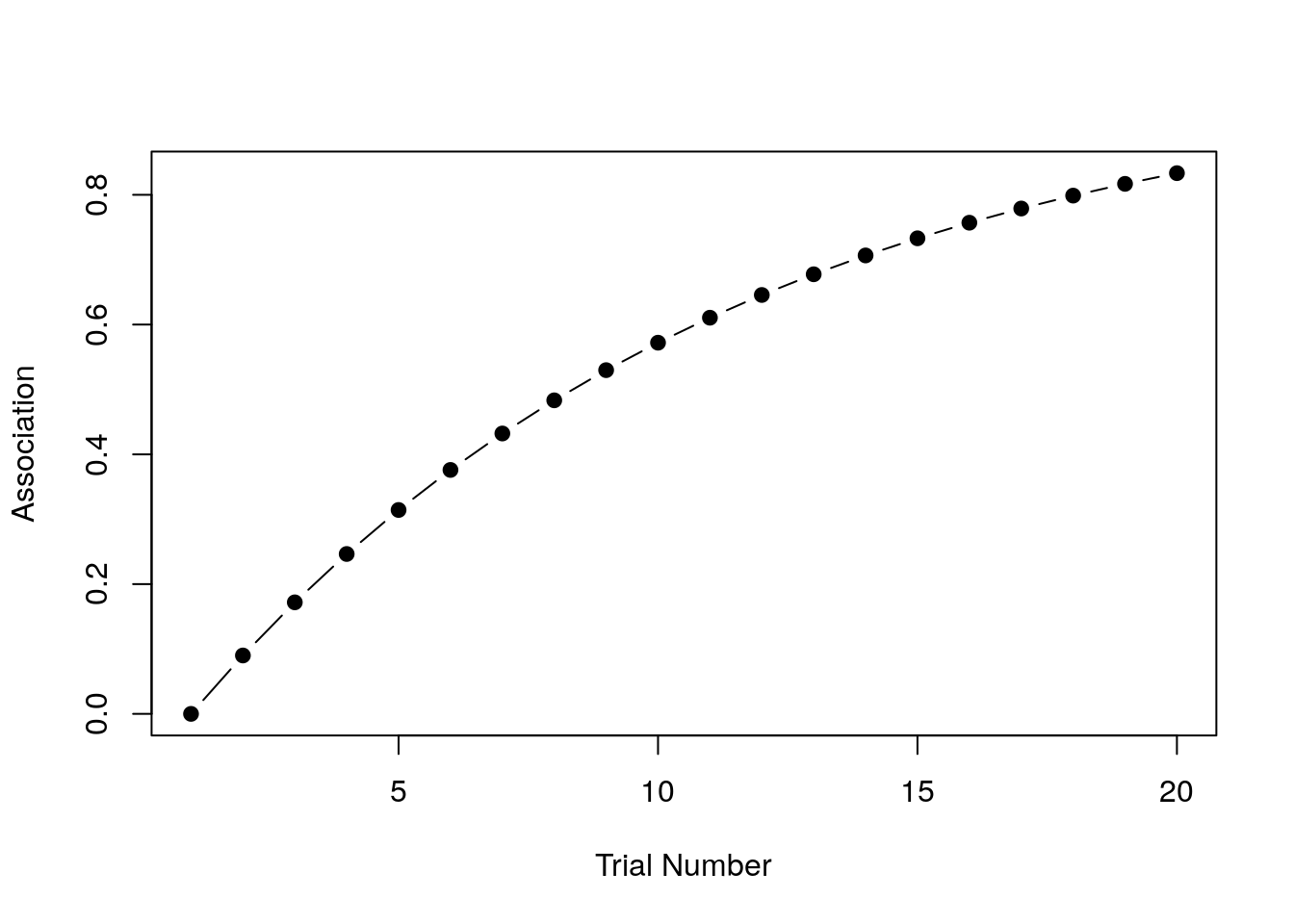
I’ve hidden the R command that produces the plot, because we haven’t covered data visualisation yet. However, if you are interested in a sneak peek, the source code for all the analyses in this section are here.

B.4.9 Extinction

For the second example, let’s consider the extinction of a learned association. What we’ll do this time is start out doing the same thing as last time. For the first 25 trials we’ll present a CS-US trial that pairs a tone with a shock (or whatever) and over that time the association for the CS will rise to match the reward “value” (\(\lambda = .3\)) linked to the US. Then for the next 25 trials we will present the CS alone with no US present. We’ll capture this by setting \(\lambda = 0\) to reflect the fact that the “value” to be predicted is now zero (i.e. no shock). For simplicity, we’ll leave the learning rate \(\beta\) the same for shock and no-shock.

Okay here goes. First, let’s set up our variables:

n_trials <- 50                
strength <- numeric(n_trials) 
lambda <- .3 # initial reward value

Now we have to set up our loop, same as before. This time around we need to include an if statement in the loop, to check whether we have moved from the learning phase (trials 1 to 25) to the extinction phase (trials 26 to 50), and adjust the value of \(\lambda\) accordingly.

for(trial in 2:n_trials) {
  
  # remove the shock after trial 25
  if(trial > 25) {
    lambda <- 0
  }
  
  # update associative strength on each trial
  strength[trial] <- update_RW(
    value = strength[trial-1],
    lambda = lambda
  )
}

What we expect to see in this situation is that after trial 25 when the shock is removed, the association strength starts to weaken because the learner is now associating the CS with no-shock (i.e. \(\lambda\) has dropped to zero and so the association \(v\) is slowly reverting to that value). Here’s the raw numbers:

print(strength)

##  [1] 0.00000000 0.02700000 0.05157000 0.07392870 0.09427512 0.11279036
##  [7] 0.12963922 0.14497169 0.15892424 0.17162106 0.18317516 0.19368940
## [13] 0.20325735 0.21196419 0.21988741 0.22709755 0.23365877 0.23962948
## [19] 0.24506283 0.25000717 0.25450653 0.25860094 0.26232685 0.26571744
## [25] 0.26880287 0.24461061 0.22259565 0.20256205 0.18433146 0.16774163
## [31] 0.15264488 0.13890684 0.12640523 0.11502876 0.10467617 0.09525531
## [37] 0.08668234 0.07888093 0.07178164 0.06532129 0.05944238 0.05409256
## [43] 0.04922423 0.04479405 0.04076259 0.03709395 0.03375550 0.03071750
## [49] 0.02795293 0.02543716

Here they are as a pretty picture:

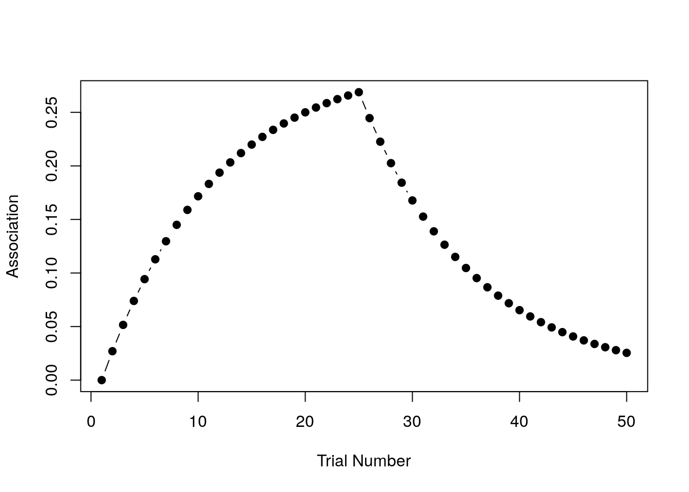
That looks right to me! Extinction is initially effective at removing the association, but it’s effectiveness declines over time, so that by the end of the task there’s still some association left.

B.4.10 Blocking

For the final example, consider a blocking paradigm. In this design we might initially pair a tone with a shock (A+ trials) for a number of trials until an association is learned. Then we present a compound stimulus AB (tone plus light) together with a shock (AB+). During the first phase, the learner quickly acquires a strong association between A and the shock, but then during the second phase they don’t learn very much about B, because A already predicts the shock.³¹

Because we are presenting a compound stimulus, the values that we pass to the update_RW function can be vectors. But that’s okay, we designed our function to be able to handle that. So let’s start by setting up our modelling exercise:

# total number of trials across 
# both phases of the task
n_trials <- 50

# vectors of zeros
strength_A <- rep(0,n_trials)
strength_B <- rep(0,n_trials)

There are two strength vectors here, one for the tone (A) and one for the light (B). Of course, during the first phase of the task the light isn’t actually present, which we can capture by setting the relevant learning rate (or salience) parameter \(\alpha\) to 0:

alpha <- c(.3, 0)

This means that at the start of the task, the model will learn about the tone but not the light. After trial 15, however, both stimuli will be present. For simplicity I’ll assume they’re equally salient, so after trial 15 the \(\alpha\) value becomes .3 for both stimuli.

As before we construct a loop over the trials:

for(trial in 2:n_trials) {
  
  # after trial 15, both stimuli are present
  if(trial > 15) alpha <- c(.3, .3)
  
  # vector of current associative strengths
  v_old <- c(strength_A[trial-1], strength_B[trial-1])
  
  # vector of new associative strengths
  v_new <- update_RW(
    value = v_old,
    alpha = alpha
   )
  
  # record the new strengths
  strength_A[trial] <- v_new[1]
  strength_B[trial] <- v_new[2]
}

It’s a little more complex this time because we have read off two strength values and pass them to the update_RW function.³² Hopefully it is clear what this code is doing.

As with the previous two examples we could print out strength_A and strength_B, but realistically no-one likes looking at long lists of numbers so let’s just draw the picture. In the plot below, the blue line shows the associative strength to A and the red line shows the associative strength to B:

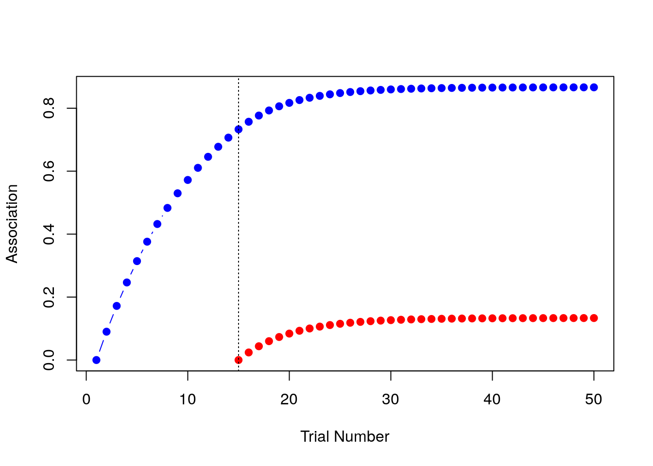
That’s the blocking effect, right there! The model learns a strong association between the tone and the shock (blue) but the association it learns between the light and the shock (red) is much weaker.

B.4.11 Done!

If you’ve been following along yourself you are now officially a computational modeller. Nice work!

There are other ways of making conditional statements in R. In particular, the ifelse function and the switch functions can be very useful in different contexts.↩
In a real blocking study there would be various control conditions but I’m not going to bother modelling those here. I just want to show how our code works for the important one!↩
In fact, we could make this code a lot simpler if we’d recorded the strengths as a matrix rather than two vectors, but since I haven’t introduced matrices yet I’ve left it in this slightly more clunky form with vectors↩